Automated Control of Cellular Neuroscience Experiments with Image Processing
By Ho-Jun Suk, MIT Media Lab and McGovern Institute, Harvard-MIT Health Sciences and Technology
Neuroscientists often study neuronal electrophysiology—the electrical activity of neurons taking place inside the brain—to gain a better understanding of the processes that may underlie specific behaviors as well as diseases related to the brain, such as schizophrenia, Alzheimer’s disease, and Parkinson’s disease.
Cell-targeted patch-clamping is a proven technique for measuring electrical activity of individual neurons, but it is extremely challenging to perform manually, especially in vivo; it requires the simultaneous operation of a two-photon microscope and a micromanipulator to guide a pipette into contact with a targeted cell in the intact brain (with the cell often moving in response to the pipette movement, thus requiring multiple pipette position adjustments to compensate for cell movements) and the application of just enough suction to break through the cell membrane (Figure 1). The handful of researchers in the world who can perform manual patch-clamping of targeted cells in vivo have a success rate of about 20%.
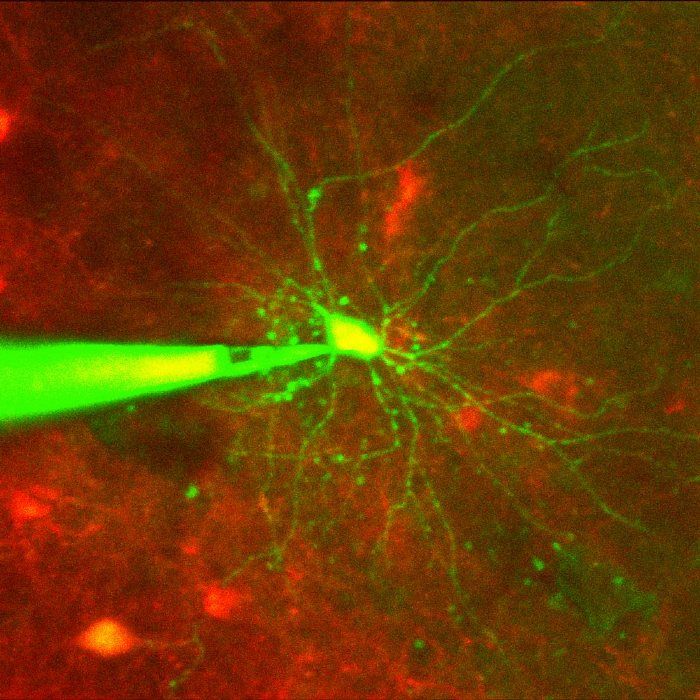
Figure 1. Measuring electrical activity in single neurons in vivo with cell-targeted patch-clamping.
Working in Edward Boyden’s research group at the MIT Media Lab and McGovern Institute, I developed a system that automates cell-targeted patch-clamping in vivo, making it possible for many more neuroscientists to apply the technique in their labs. Implemented as a MATLAB® app, my Imagepatcher software processes images from a two-photon microscope, sends commands to a four-axis micromanipulator, and applies suction by controlling electronic pressure regulators and valves. In the living mouse brain, the initial implementation of the Imagepatcher system performed as well as experienced neuroscientists, and with success rates that matched or exceeded theirs.
How Manual Patch-Clamping Works
Cell-targeted patch-clamping is a multistage process that begins when the tip of a pipette is moved into contact with the targeted cell (Figure 2). To complete this first stage manually, the researcher uses a two-photon microscope to identify the targeted cell and a micromanipulator to maneuver the pipette tip into the field of view. Operating the microscope with one hand and the micromanipulator with the other, the researcher gradually moves the pipette tip closer to the targeted cell, carefully compensating for cell movements as the pipette tip approaches the cell membrane, with multiple rounds of microscope focus and field-of-view adjustments.

Figure 2. Stages in the cell-targeted patch-clamping process. ACSF = artificial cerebrospinal fluid; red = fluorescent cells; green = patch pipette filled with fluorescent dye; light red = laser for two-photon imaging; black solid arrows = pipette movements; black dotted arrow = cell movement; yellow = target cell filled with the fluorescent dye from the pipette.
A sudden change in the electrical resistance measured at the pipette tip confirms that the tip is in contact with the cell. At this point, the researcher must quickly change focus from the micromanipulator to a syringe. The syringe, whose tip is connected to the back of the pipette via a hollow tube, is used to apply suction to the pipette to help establish a gigaseal, a tight seal between the tip and the patch of cell membrane in contact with the pipette tip; giga refers to resistance of greater than one gigaohm (1 GΩ). The researcher then applies a series of suction pulses to achieve break in, a rupture of the cell membrane patch that provides access to the inside of the cell. This state, known as whole-cell configuration, enables high-quality recordings of the cell’s electrical activity. To achieve high-quality recordings, researchers must perform the entire procedure with as little damage to the cell as possible.
Accessing and Controlling Lab Equipment from Within MATLAB
To automate the numerous manual operations involved in patch-clamping, I needed an interface between MATLAB and each of the three instruments involved: the two-photon microscope, the micromanipulator, and the electronic pressure regulators and valves that control the pressure at the pipette tip (Figure 3). The interface to the microscope was provided by ScanImage, an open-source software package for microscope control maintained by Vidrio Technologies. I used ScanImage to control all aspects of image acquisition, including when and how to capture images from the microscope for processing in MATLAB. The interface to the micromanipulator was provided as a library by the manufacturer (Sensapex). I used this library to control the motion of the pipette with a uniform speed from within MATLAB. I developed the interface to the regulators and valves using a National Instruments data acquisition (DAQ) board and Instrument Control Toolbox™.

Figure 3. Imagepatcher setup.
Implementing Imagepatcher Control Loops
The Imagepatcher software includes three main control loops. Each loop is run in MATLAB. The first manages the movement of the pipette until its tip contacts the targeted neuron, the second applies suction to form a gigaseal, and the third applies suction pulses to achieve break-in. During a patch-clamping procedure, the Imagepatcher software runs these control loops autonomously. A MATLAB based interface enables the researcher to manage and monitor the procedure (Figure 4).

Figure 4. The Imagepatcher interface.
The algorithm for the first control loop acquires an image from the microscope, analyzes it to identify the cell, calculates the offset between the cell and the pipette tip, and sends commands to the micromanipulator to move the pipette closer to the cell. These steps are repeated until the pipette has reached its target, signaled by an abrupt change in electrical resistance measured at the pipette tip.
Within this loop, I invoked image processing functions to analyze the images generated by the microscope. First, I use a 2D Wiener filter to remove photon noise, which appears as high-intensity speckles in the image. Next, I apply a thresholding function to produce a binary version of the image that isolates the fluorescently labeled cell. I then perform morphological operations on the binary image to determine the centroid of the cell—the point within the cell boundary that I target with the pipette. I use a similar procedure, before the start of the loop, to isolate the pipette in the image and identify its tip (Figure 5). This initial location of the tip is used to calculate the tip position following pipette movements within the loop. After computing the offset between the cell centroid and the pipette tip in three dimensions, the algorithm generates the micromanipulator commands needed to move the pipette and sends the commands to the micromanipulator via a serial interface.
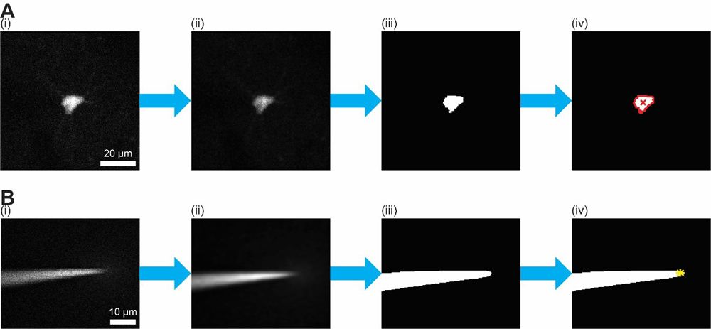
Figure 5. Image processing steps for detecting (A) the centroid of a target cell and (B) the tip of a pipette, showing (i) the raw microscope image, (ii) the filtered image, (iii) the binary image, and (iv) the overlay of the binary image with the detected features. Red outline = outline of the cell; red x = centroid of the cell; yellow star = tip of the pipette.
Once the pipette reaches the cell, Imagepatcher enters the pressure control loop. Here, the algorithm creates pressure at the pipette tip by using MATLAB and Data Acquisition Toolbox™ to generate analog signals for the setup’s three electronic pressure regulators and digital signals for its four electronic valves. The algorithm dynamically changes pressure until the resistance measured at the tip reaches 1 GΩ. The pressure control algorithm uses heuristics to speed up the formation of a gigaseal—for example, if the measured resistance is well below 1 GΩ and rising slowly, the algorithm increases the suction significantly, whereas if the resistance is steadily rising, it maintains the existing pressure and waits for the gigaseal to form.
The third and final control loop is used to break into the cell membrane. Originally, Imagepatcher kicked off this loop automatically after the gigaseal was achieved, but colleagues pointed out that some researchers prefer to take recordings before break-in (i.e., cell-attached recordings). Cell-attached recordings do not provide the same level of information as whole-cell recordings (e.g., sub-threshold activity), but some studies require recordings from an intact cell. To accommodate this requirement, Imagepatcher is configured to pause and wait for operator confirmation before proceeding with the third control loop.
To initiate break-in, Imagepatcher applies a series of suction pulses with increasing pressure, while again monitoring the resistance measured at the pipette’s tip. When the cell membrane ruptures, the measured resistance falls from more than 1 GΩ to a few hundred megaohms. When break-in is achieved, Imagepatcher halts suction, and the researcher can begin recording.
Initial Results and Planned Enhancements
The first version of Imagepatcher matches or slightly surpasses the success rate reported by experienced researchers, achieving whole-cell configuration about 20–22% of the time. The 10 minutes or so that Imagepatcher takes to complete a patch-clamping procedure is comparable to the time required by those researchers. The length of recordings made following automated patch-clamping (on average, about 15 minutes) and their quality were comparable to those of recordings made after manual patch-clamping procedures, suggesting that Imagepatcher does not damage the cell any more than a manual patch- clamping procedure would. Most importantly, Imagepatcher provides uniformity and consistency that cannot be matched by manual methods, enabling many more researchers to perform the procedure reliably. In fact, seven labs worldwide have already expressed interest in using Imagepatcher.
I plan to implement enhancements that will improve both the speed and the success rate of Imagepatcher by capitalizing on the hardware’s ability to perform techniques that cannot be performed manually, such as the precise application of suction pulse patterns.
Published 2018