Normal Distribution
Overview
The normal distribution, sometimes called the Gaussian distribution, is a two-parameter family of curves. The usual justification for using the normal distribution for modeling is the Central Limit theorem, which states (roughly) that the sum of independent samples from any distribution with finite mean and variance converges to the normal distribution as the sample size goes to infinity.
Statistics and Machine Learning Toolbox™ offers several ways to work with the normal distribution.
Create a probability distribution object
NormalDistributionby fitting a probability distribution to sample data (fitdist) or by specifying parameter values (makedist). Then, use object functions to evaluate the distribution, generate random numbers, and so on.Work with the normal distribution interactively by using the Distribution Fitter app. You can export an object from the app and use the object functions.
Use distribution-specific functions (
normcdf,normpdf,norminv,normlike,normstat,normfit,normrnd) with specified distribution parameters. The distribution-specific functions can accept parameters of multiple normal distributions.Use generic distribution functions (
cdf,icdf,pdf,random) with a specified distribution name ('Normal') and parameters.
Parameters
The normal distribution uses these parameters.
| Parameter | Description | Support |
|---|---|---|
mu (μ) | Mean | |
sigma (σ) | Standard deviation |
The standard normal distribution has zero mean and unit standard deviation. If z is standard normal, then σz + µ is also normal with mean µ and standard deviation σ. Conversely, if x is normal with mean µ and standard deviation σ, then z = (x – µ) / σ is standard normal.
Parameter Estimation
The maximum likelihood estimates (MLEs) are the parameter estimates that maximize the likelihood function. The maximum likelihood estimators of μ and σ2 for the normal distribution, respectively, are
and
is the sample mean for samples x1, x2, …, xn. The sample mean is an unbiased estimator of the parameter μ. However, s2MLE is a biased estimator of the parameter σ2, meaning that its expected value does not equal the parameter.
The minimum variance unbiased estimator (MVUE) is commonly used to estimate the parameters of the normal distribution. The MVUE is the estimator that has the minimum variance of all unbiased estimators of a parameter. The MVUEs of the parameters μ and σ2 for the normal distribution are the sample mean x̄ and sample variance s2, respectively.
To fit the normal distribution to data and find the parameter estimates, use
normfit, fitdist, or mle.
For uncensored data,
normfitandfitdistfind the unbiased estimates, andmlefinds the maximum likelihood estimates.For censored data,
normfit,fitdist, andmlefind the maximum likelihood estimates.
Unlike normfit and mle,
which return parameter estimates, fitdist returns the
fitted probability distribution object NormalDistribution. The object
properties mu and sigma store the
parameter estimates.
For an example, see Fit Normal Distribution Object.
Probability Density Function
The normal probability density function (pdf) is
The likelihood function is the pdf viewed as a function of the
parameters. The maximum likelihood estimates (MLEs) are the parameter estimates that
maximize the likelihood function for fixed values of x.
For an example, see Compute and Plot the Normal Distribution pdf.
Cumulative Distribution Function
The normal cumulative distribution function (cdf) is
p is the probability that a single observation from a normal distribution with parameters μ and σ falls in the interval (-∞,x].
The standard normal cumulative distribution function Φ(x) is functionally related to the error function erf.
where
For an example, see Plot Standard Normal Distribution cdf
Examples
Fit Normal Distribution Object
Load the sample data and create a vector containing the first column of student exam grade data.
load examgrades
x = grades(:,1);
Create a normal distribution object by fitting it to the data.
pd = fitdist(x,'Normal')pd =
NormalDistribution
Normal distribution
mu = 75.0083 [73.4321, 76.5846]
sigma = 8.7202 [7.7391, 9.98843]
The intervals next to the parameter estimates are the 95% confidence intervals for the distribution parameters.
Estimate Parameters
Estimate normal distribution parameters (mean and standard deviation) by using the normfit function.
Load the sample data and create a vector containing the first column of student exam grade data.
load examgrades
x = grades(:,1);
Find the parameter estimates and the 95% confidence intervals.
[mu,s,muci,sci] = normfit(x)
mu = 75.0083
s = 8.7202
muci = 2×1

   73.4321
   76.5846
sci = 2×1

    7.7391
    9.9884
The normfit function returns the minimum variance unbiased estimator (MVUE) for , the square root of the MVUE for , and 95% confidence intervals for and .
Note that the square of s is the MVUE of the variance.
s^2
ans = 76.0419
Compute and Plot the Normal Distribution pdf
Compute the pdf of a standard normal distribution, with parameters equal to 0 and equal to 1.
x = [-3:.1:3];
y = normpdf(x,0,1);
Plot the pdf.
plot(x,y)

Plot Standard Normal Distribution cdf
Create a standard normal distribution object.
pd = makedist('Normal')pd =
NormalDistribution
Normal distribution
mu = 0
sigma = 1
Specify the x values and compute the cdf.
x = -3:.1:3;
p = cdf(pd,x);
Plot the cdf of the standard normal distribution.
plot(x,p)

Compare Gamma and Normal Distribution pdfs
The gamma distribution has the shape parameter and the scale parameter . For a large , the gamma distribution closely approximates the normal distribution with mean and variance .
Compute the pdf of a gamma distribution with parameters a = 100 and b = 5.
a = 100;
b = 5;
x = 250:750;
y_gam = gampdf(x,a,b);
For comparison, compute the mean, standard deviation, and pdf of the normal distribution that gamma approximates.
mu = a*b
mu = 500
sigma = sqrt(a*b^2)
sigma = 50
y_norm = normpdf(x,mu,sigma);
Plot the pdfs of the gamma distribution and the normal distribution on the same figure.
plot(x,y_gam,'-',x,y_norm,'-.')
title('Gamma and Normal pdfs')
xlabel('Observation')
ylabel('Probability Density')
legend('Gamma Distribution','Normal Distribution')
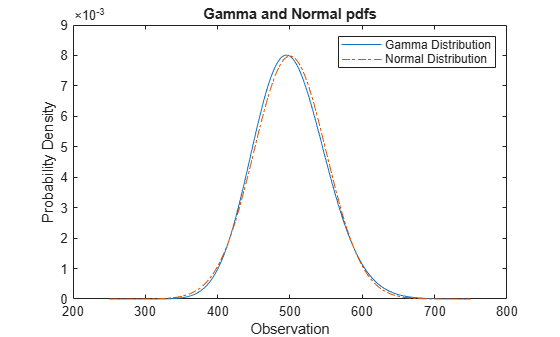
The pdf of the normal distribution approximates the pdf of the gamma distribution.
Relationship Between Normal and Lognormal Distributions
If X follows the lognormal distribution with parameters µ and σ, then log(X) follows the normal distribution with mean µ and standard deviation σ. Use distribution objects to inspect the relationship between normal and lognormal distributions.
Create a lognormal distribution object by specifying the parameter values.
pd = makedist('Lognormal','mu',5,'sigma',2)
pd =
  LognormalDistribution

  Lognormal distribution
       mu = 5
    sigma = 2
Compute the mean of the lognormal distribution.
mean(pd)
ans = 1.0966e+03
The mean of the lognormal distribution is not equal to the mu parameter. The mean of the logarithmic values is equal to mu. Confirm this relationship by generating random numbers.
Generate random numbers from the lognormal distribution and compute their log values.
rng('default');  % For reproducibility
x = random(pd,10000,1);
logx = log(x);
Compute the mean of the logarithmic values.
m = mean(logx)
m = 5.0033
The mean of the log of x is close to the mu parameter of x, because x has a lognormal distribution.
Construct a histogram of logx with a normal distribution fit.
histfit(logx)

The plot shows that the log values of x are normally distributed.
histfit uses fitdist to fit a distribution to data. Use fitdist to obtain parameters used in fitting.
pd_normal = fitdist(logx,'Normal')pd_normal =
NormalDistribution
Normal distribution
mu = 5.00332 [4.96445, 5.04219]
sigma = 1.98296 [1.95585, 2.01083]
The estimated normal distribution parameters are close to the lognormal distribution parameters 5 and 2.
Compare Student's t and Normal Distribution pdfs
The Student’s t distribution is a family of curves depending on a single parameter ν (the degrees of freedom). As the degrees of freedom ν approach infinity, the t distribution approaches the standard normal distribution.
Compute the pdfs for the Student's t distribution with the parameter nu = 5 and the Student's t distribution with the parameter nu = 15.
x = [-5:0.1:5];
y1 = tpdf(x,5);
y2 = tpdf(x,15);
Compute the pdf for a standard normal distribution.
z = normpdf(x,0,1);
Plot the Student's t pdfs and the standard normal pdf on the same figure.
plot(x,y1,'-.',x,y2,'--',x,z,'-')
legend('Student''s t Distribution with \nu=5', ...
    'Student''s t Distribution with \nu=15', ...
    'Standard Normal Distribution','Location','best')
xlabel('Observation')
ylabel('Probability Density')
title('Student''s t and Standard Normal pdfs')

The standard normal pdf has shorter tails than the Student's t pdfs.
Related Distributions
Binomial Distribution — The binomial distribution models the total number of successes in n repeated trials with the probability of success p. As n increases, the binomial distribution can be approximated by a normal distribution with µ = np and σ2 = np(1–p). See Compare Binomial and Normal Distribution pdfs.
Birnbaum-Saunders Distribution — If x has a Birnbaum-Saunders distribution with parameters β and γ, then
has a standard normal distribution.
Chi-Square Distribution — The chi-square distribution is the distribution of the sum of squared, independent, standard normal random variables. If a set of n observations is normally distributed with variance σ2, and s2 is the sample variance, then (n–1)s2/σ2 has a chi-square distribution with n–1 degrees of freedom. The
normfitfunction uses this relationship to calculate confidence intervals for the estimate of the normal parameter σ2 .Extreme Value Distribution — The extreme value distribution is appropriate for modeling the smallest or largest value from a distribution whose tails decay exponentially fast, such as, the normal distribution.
Gamma Distribution — The gamma distribution has the shape parameter a and the scale parameter b. For a large a, the gamma distribution closely approximates the normal distribution with mean μ = ab and variance σ2 = ab2. The gamma distribution has density only for positive real numbers. See Compare Gamma and Normal Distribution pdfs.
Half-Normal Distribution — The half-normal distribution is a special case of the folded normal and truncated normal distributions. If a random variable
Zhas a standard normal distribution, then has a half-normal distribution with parameters μ and σ.Logistic Distribution — The logistic distribution is used for growth models and in logistic regression. It has longer tails and a higher kurtosis than the normal distribution.
Lognormal Distribution — If X follows the lognormal distribution with parameters µ and σ, then log(X) follows the normal distribution with mean µ and standard deviation σ. See Relationship Between Normal and Lognormal Distributions.
Multivariate Normal Distribution — The multivariate normal distribution is a generalization of the univariate normal to two or more variables. It is a distribution for random vectors of correlated variables, in which each element has a univariate normal distribution. In the simplest case, there is no correlation among variables, and elements of the vectors are independent, univariate normal random variables.
Poisson Distribution — The Poisson distribution is a one-parameter discrete distribution that takes nonnegative integer values. The parameter, λ, is both the mean and the variance of the distribution. As λ increase, the Poisson distribution can be approximated by a normal distribution with µ = λ and σ2 = λ.
Rayleigh Distribution — The Rayleigh distribution is a special case of the Weibull distribution with applications in communications theory. If the component velocities of a particle in the x and y directions are two independent normal random variables with zero means and equal variances, then the distance the particle travels per unit time follows the Rayleigh distribution.
Stable Distribution — The normal distribution is a special case of the stable distribution. The stable distribution with the first shape parameter α = 2 corresponds to the normal distribution.
Student's t Distribution — The Student’s t distribution is a family of curves depending on a single parameter ν (the degrees of freedom). As the degrees of freedom ν goes to infinity, the t distribution approaches the standard normal distribution. See Compare Student's t and Normal Distribution pdfs.
If x is a random sample of size n from a normal distribution with mean μ, then the statistic
where is the sample mean and s is the sample standard deviation, has the Student's t distribution with n–1 degrees of freedom.
t Location-Scale Distribution — The t location-scale distribution is useful for modeling data distributions with heavier tails (more prone to outliers) than the normal distribution. It approaches the normal distribution as the shape parameter ν approaches infinity.
References
[1] Abramowitz, M., and I. A. Stegun. Handbook of Mathematical Functions. New York: Dover, 1964.
[2] Evans, M., N. Hastings, and B. Peacock. Statistical Distributions. 2nd ed. Hoboken, NJ: John Wiley & Sons, Inc., 1993.
[3] Lawless, J. F. Statistical Models and Methods for Lifetime Data. Hoboken, NJ: Wiley-Interscience, 1982.
[4] Marsaglia, G., and W. W. Tsang. “A Fast, Easily Implemented Method for Sampling from Decreasing or Symmetric Unimodal Density Functions.” SIAM Journal on Scientific and Statistical Computing. Vol. 5, Number 2, 1984, pp. 349–359.
[5] Meeker, W. Q., and L. A. Escobar. Statistical Methods for Reliability Data. Hoboken, NJ: John Wiley & Sons, Inc., 1998.
See Also
NormalDistribution | normcdf | normpdf | norminv | normlike | normstat | normfit | normrnd | erf
Related Topics
You can also select a web site from the following list:
Americas
- América Latina (Español)
- Canada (English)
- United States (English)
Europe
- Belgium (English)
- Denmark (English)
- Deutschland (Deutsch)
- España (Español)
- Finland (English)
- France (Français)
- Ireland (English)
- Italia (Italiano)
- Luxembourg (English)
- Netherlands (English)
- Norway (English)
- Österreich (Deutsch)
- Portugal (English)
- Sweden (English)
- Switzerland
- United Kingdom (English)